enDAQ Custom Analysis

Introduction

This notebook and accompanying webinar was developed and released by the enDAQ team. This is the fifth “chapter” of our series on Python for Mechanical Engineers:

1. Get Started with Python

   • Blog: Get Started with Python: Why and How Mechanical Engineers Should Make the Switch

2. Introduction to Numpy & Pandas for Data Analysis

3. Introduction to Plotly for Plotting Data

4. Introduction of the enDAQ Library

   • There are lots of examples in this!

5. More Examples! (Today’s Webinar)

   • Frequency Analysis (FFTs and PSDs)

   • Simple Shock Response Spectrums

   • Peak Analysis

   • Preview endaq.batch

To sign up for future webinars and watch previous ones, visit our webinars page.

Installation

Available on PyPi via: > pip install endaq

For the most recent features that are still under development, you can also use pip to install endaq directly from GitHub: > pip install git+https://github.com/MideTechnology/endaq-python.git@development

!pip install -q endaq
!pip install -q kaleido #this is for rendering images with plotly
exit() #needed in Colab because they pre-load some libraries, wouldn't be neccessary if running locally

     |████████████████████████████████| 71 kB 3.0 MB/s
     |████████████████████████████████| 11.3 MB 13.0 MB/s
     |████████████████████████████████| 62 kB 749 kB/s
     |████████████████████████████████| 38.1 MB 1.3 MB/s
     |████████████████████████████████| 93 kB 1.0 MB/s
     |████████████████████████████████| 83 kB 1.0 MB/s
     |████████████████████████████████| 25.3 MB 51.8 MB/s
ERROR: pip's dependency resolver does not currently take into account all the packages that are installed. This behaviour is the source of the following dependency conflicts.
google-colab 1.0.0 requires pandas~=1.1.0; python_version >= "3.0", but you have pandas 1.3.4 which is incompatible.
google-colab 1.0.0 requires requests~=2.23.0, but you have requests 2.26.0 which is incompatible.
datascience 0.10.6 requires folium==0.2.1, but you have folium 0.8.3 which is incompatible.
albumentations 0.1.12 requires imgaug<0.2.7,>=0.2.5, but you have imgaug 0.2.9 which is incompatible.
     |████████████████████████████████| 79.9 MB 1.2 MB/s

import endaq

endaq.plot.utilities.set_theme(theme='endaq')

import plotly.express as px
import plotly.graph_objects as go
import plotly.io as pio; pio.renderers.default = "iframe"
import pandas as pd
import numpy as np
import scipy

PSDs & FFTs

Simple Sine Wave

time = np.linspace(0,2,200,endpoint=False)

sine_waves = pd.DataFrame(index=time)
sine_waves['0.8g @ 2 Hz'] = 0.8*np.sin(2*np.pi*2 * time)
sine_waves['1g @ 3 Hz'] = np.sin(2*np.pi*3 * time)
sine_waves['0.6g @ 5 Hz'] = 0.6*np.sin(2*np.pi*5 * time)
sine_waves['0.5g @ 4 & 6 Hz'] = 0.5*np.sin(2*np.pi*4 * time) + 0.5*np.sin(2*np.pi*6 * time)
sine_waves['0.3g @ 7 Hz'] = 0.3*np.sin(2*np.pi*7 * time)

sine_waves

	0.8g @ 2 Hz	1g @ 3 Hz	0.6g @ 5 Hz	0.5g @ 4 & 6 Hz	0.3g @ 7 Hz
0.00	0.000000	0.000000	0.000000	0.000000	0.000000
0.01	0.100267	0.187381	0.185410	0.308407	0.127734
0.02	0.198952	0.368125	0.352671	0.583150	0.231154
0.03	0.294500	0.535827	0.485410	0.794687	0.290575
0.04	0.385403	0.684547	0.570634	0.921177	0.294686
...	...	...	...	...	...
1.95	-0.470228	-0.809017	-0.600000	-0.951057	-0.242705
1.96	-0.385403	-0.684547	-0.570634	-0.921177	-0.294686
1.97	-0.294500	-0.535827	-0.485410	-0.794687	-0.290575
1.98	-0.198952	-0.368125	-0.352671	-0.583150	-0.231154
1.99	-0.100267	-0.187381	-0.185410	-0.308407	-0.127734

200 rows × 5 columns

fig = px.line(sine_waves)
fig.update_layout(
    title_text='Comparison of Fabricated Sine Waves',
    yaxis_title_text='Acceleration (g)',
    xaxis_title_text='Time (s)',
    legend_title_text=''
)

Now to compute the PSD on this using endaq.calc.psd.welch(), see docs

psd = endaq.calc.psd.welch(sine_waves, bin_width=0.5)

fig = px.line(psd)
fig.update_layout(
    title_text='Comparison of the PSD of Two Fabricated Sine Waves',
    yaxis_title_text='Acceleration (g^2/Hz)',
    xaxis_title_text='Frequency (Hz)',
    xaxis_type='log',
    legend_title_text=''
)

PSDs are the more appropriate way to analyze vibration data for a number of reasons (see blog) but we typically see people want to see the FFT because it’s units are easier to intuitively understand.

In my experience the best way to do this is to compute a PSD using our function with a few modifications: - Use scaling as parseval which means it is g^2 instead of g^2/Hz - Use a boxcar window so in effect there is no windowing - Define a very fine bin width - Set the overlap between FFTs to 0 (not necessary if the bin width is small enough) - Scale from g^2 as RMS to g-peak via **2 * (2**0.5)

fft = endaq.calc.psd.welch(
    sine_waves,
    scaling='parseval',
    window='boxcar',
    noverlap=0,
    bin_width=0.1,
)
fft = fft**0.5 * (2**0.5) #scale from g^2 as RMS to g-peak

fig = px.line(fft)
fig.update_layout(
    title_text='Comparison of the FFT (from PSD) of Two Fabricated Sine Waves',
    yaxis_title_text='Acceleration (g)',
    xaxis_title_text='Frequency (Hz)',
    xaxis_type='log',
    legend_title_text='',
    template='endaq_light'
)

/usr/local/lib/python3.7/dist-packages/scipy/signal/spectral.py:1966: UserWarning:

nperseg = 1000 is greater than input length  = 200, using nperseg = 200

Real Sine Wave

Let’s load a IDE file with get_doc docs.

doc = endaq.ide.get_doc('https://info.endaq.com/hubfs/100Hz_shake_cal.ide')
endaq.ide.get_channel_table(doc)

	channel	name	type	units	start	end	duration	samples	rate
0	8.0	X (100g)	Acceleration	g	00:00.0218	00:25.0532	00:25.0314	126575	5000.07 Hz
1	8.1	Y (100g)	Acceleration	g	00:00.0218	00:25.0532	00:25.0314	126575	5000.07 Hz
2	8.2	Z (100g)	Acceleration	g	00:00.0218	00:25.0532	00:25.0314	126575	5000.07 Hz
3	80.0	X (40g)	Acceleration	g	00:00.0218	00:25.0547	00:25.0328	100934	3985.00 Hz
4	80.1	Y (40g)	Acceleration	g	00:00.0218	00:25.0547	00:25.0328	100934	3985.00 Hz
5	80.2	Z (40g)	Acceleration	g	00:00.0218	00:25.0547	00:25.0328	100934	3985.00 Hz
6	36.0	Pressure/Temperature:00	Pressure	Pa	00:00.0217	00:25.0702	00:25.0485	27	1.06 Hz
7	36.1	Pressure/Temperature:01	Temperature	°C	00:00.0217	00:25.0702	00:25.0485	27	1.06 Hz
8	70.0	X	Quaternion	q	00:00.0284	00:24.0682	00:24.0397	2424	99.35 Hz
9	70.1	Y	Quaternion	q	00:00.0284	00:24.0682	00:24.0397	2424	99.35 Hz
10	70.2	Z	Quaternion	q	00:00.0284	00:24.0682	00:24.0397	2424	99.35 Hz
11	70.3	W	Quaternion	q	00:00.0284	00:24.0682	00:24.0397	2424	99.35 Hz
12	59.0	Control Pad Pressure	Pressure	Pa	00:00.0251	00:25.0399	00:25.0148	252	10.02 Hz
13	59.1	Control Pad Temperature	Temperature	°C	00:00.0251	00:25.0399	00:25.0148	252	10.02 Hz
14	59.2	Relative Humidity	Relative Humidity	RH	00:00.0251	00:25.0399	00:25.0148	252	10.02 Hz
15	76.0	Lux	Light	Ill	00:00.0000	00:25.0278	00:25.0278	100	3.96 Hz
16	76.1	UV	Light	Index	00:00.0000	00:25.0278	00:25.0278	100	3.96 Hz

Now get the actual data out of one channel with to_pandas() docs.

Then generate a plot with rolling_min_max_envelope() (docs) that will instead of plotting all data points make a shaded plot which will look identical to plotting all points but be more responsive and faster (not entirely necessary on this dataset, but becomes so with larger ones).

accel = endaq.ide.to_pandas(doc.channels[80], time_mode='seconds')
accel = accel-accel.median() #remove DC offset
endaq.plot.rolling_min_max_envelope(
    accel,
    plot_as_bars=True,
    desired_num_points=1000,
    opacity=0.7
)

Here we’ll plot the raw data around the peak event with around_peak() docs.

endaq.plot.around_peak(accel, num=500)

fft = endaq.calc.psd.welch(
    accel[4.5:9.5], #just do it in time of first dwell
    scaling='parseval',
    window='boxcar',
    noverlap=0,
    bin_width=0.5,
)
fft = fft**0.5 * (2**0.5) #scale from g^2 as RMS to g-peak

fig = px.line(fft[:500])
fig.update_layout(
    title_text='FFT (from PSD) of Real World 10.3g Sine Wave',
    yaxis_title_text='Acceleration (g)',
    xaxis_title_text='Frequency (Hz)',
    legend_title_text='',
)

Comparing FFT Options

FFT Option Overview

There are a lot of different ways to compute a FFT in Python. I’ve been using Welch’s method so far but I want to compare that to some other more “direct” methods. So let’s compare them! First let’s conveniently wrap our manipulation of Welch’s method PSD into a FFT inside a function.

def welch_fft(df, bin_width=0.5):
  fft = endaq.calc.psd.welch(df, bin_width=bin_width, scaling='parseval', window='boxcar', noverlap=0)
  return fft**0.5 * (2**0.5) #scale from g^2 as RMS to g-peak

Now let’s wrap something around Numpy’s FFT functions for a real discrete Fourier transform.

Notice here we actually have phase information! So we’ll return that too.

def numpy_fft(df):
  """
  Using Numpy's rfft functions compute a discrete Fourier Transform
  """
  freq = np.fft.rfftfreq(len(df), d=endaq.calc.utils.sample_spacing(df))
  df_fft = pd.DataFrame(
    np.fft.rfft(df.to_numpy(), axis=0),
    index=pd.Series(freq, name="frequency (Hz)"),
    columns=df.columns
  )

  df_mag = df_fft.apply(np.abs, raw=True) / len(df_fft)
  df_phase = df_fft.apply(np.angle, raw=True)

  return df_mag, df_phase

Now we will use the FFTW algorithm which is available in the pyFFTW library under a GPL license (which makes it potentially difficult for us to use because we use the more premissive MIT license).

First let’s download it.

!pip install -q pyfftw

     |████████████████████████████████| 2.6 MB 5.3 MB/s

Now let’s use it in a function which allows for a drop-in replacement to the Numpy code. This algorithm is generally regarded as the fatest for computing discrete Fourier transforms - so we’ll put it to the test!

import pyfftw

def fftw_fft(df):
  """
  Using the FFTW algorithm, compute a discrete Fourier Transform
  """
  freq = pyfftw.interfaces.numpy_fft.rfftfreq(len(df), d=endaq.calc.utils.sample_spacing(df))
  df_fft = pd.DataFrame(
    pyfftw.interfaces.numpy_fft.rfft(df.to_numpy(), axis=0),
    index=pd.Series(freq, name="frequency (Hz)"),
    columns=df.columns
  )

  df_mag = df_fft.apply(np.abs, raw=True) / len(df_fft)
  df_phase = df_fft.apply(np.angle, raw=True)

  return df_mag, df_phase

Now let’s see a FFT result with this library. Note though this will be relatively large to plot…

fft, phase = fftw_fft(accel[4.5:9.5])

fig = px.line(fft[80:120])
fig.update_layout(
    title_text='FFT using FFTW of Real World 10.3g Sine Wave',
    yaxis_title_text='Acceleration (g)',
    xaxis_title_text='Frequency (Hz)',
    legend_title_text='',
)

Remember one of the benefits of the DFT is to get phase. Although not particularly useful for this dataset let’s plot it, notice the shift for the Z axis at the drive frequency.

fig = px.line(phase[80:120])
fig.update_layout(
    title_text='Phase using FFTW of Real World 10.3g Sine Wave',
    yaxis_title_text='Phase Angle (radians)',
    xaxis_title_text='Frequency (Hz)',
    legend_title_text='',
)

FFT Option Comparison

Now let’s do the fun part to compare the three approaches! First let’s make a sine wave with a bit over 1M points.

time = np.linspace(0,200,2**20,endpoint=False)

sine_waves = pd.DataFrame(index=time)
sine_waves['10g @ 100 Hz'] = 10*np.sin(2*np.pi*100 * time)
sine_waves['8g @ 99 Hz'] = 8*np.sin(2*np.pi*99 * time)
sine_waves['6g @ 100.25 Hz'] = 6*np.sin(2*np.pi*100.25 * time)

fig = px.line(sine_waves[:0.01])
fig.update_layout(
    title_text='Comparison of Fabricated Sine Waves',
    yaxis_title_text='Acceleration (g)',
    xaxis_title_text='Time (s)',
    legend_title_text=''
)

from time import process_time
import timeit
pyfftw.forget_wisdom() #FFTW will be faster on subsequent runs

lengths = [2**14, 16411, 2**17, 131101, 2**20, 1000003]

ffts = pd.DataFrame()
times = pd.DataFrame()
def melt_fft(fft,name,L):
  fft =  fft.reset_index().melt(id_vars='frequency (Hz)')
  fft['Algo'] = name
  fft['Length'] = L
  return fft

def time_fft(func):
    return np.array(timeit.repeat(func, number=1, repeat=10)).mean()

def time_pyfftw(x, threads=1):
    pyfftw.forget_wisdom()
    rfft = pyfftw.builders.rfft(x, threads=threads, auto_align_input=True)
    rfft()
    return np.array(timeit.repeat(lambda: rfft(), number=1, repeat=10)).mean()

for L in lengths:
  x = sine_waves.iloc[:L, 0].to_numpy()

  t1 = process_time()
  wfft_bin = welch_fft(sine_waves.iloc[:L], bin_width=0.5)

  t2 = process_time()
  wfft = welch_fft(sine_waves.iloc[:L], bin_width=1/(L*endaq.calc.utils.sample_spacing(sine_waves)))

  t3 = process_time()
  nfft, phase = numpy_fft(sine_waves.iloc[:L])

  t4 = process_time()
  fftw, phase = fftw_fft(sine_waves.iloc[:L])

  t5 = process_time()

  times_t = pd.DataFrame(
      {'Welch w/ 0.5 Hz Bin':t2-t1,
       'Welch': t3-t2,
       'Numpy':t4-t3,
       'FFTW':t5-t4,
       'Numpy - No OH': time_fft(lambda: np.fft.rfft(x)),
       'FFTW - No OH': time_pyfftw(x, threads=1)
      },
      index=pd.Series([L],name='Length')
  )
  times = pd.concat([times,times_t.reset_index().melt(id_vars='Length')])

  wfft_bin = melt_fft(wfft_bin.copy(),'Welch w/ 0.5 Hz Bin',L)
  wfft = melt_fft(wfft.copy(),'Welch',L)
  nfft = melt_fft(nfft.copy(),'Numpy',L)
  fftw = melt_fft(fftw.copy(),'FFTW',L)

  ffts = pd.concat([ffts,wfft_bin,wfft,nfft,fftw])

times['str_len'] = times['Length'].astype('str')
fig = px.bar(
    times,
    x='str_len',
    y='value',
    color='variable',
    log_y=True,
    barmode='group',
    labels={'value':'Computation Time (s)','str_len':'Array Length','variable':''}
)
fig.show()

fig = px.scatter(
    times,
    x='str_len',
    y='value',
    color='variable',
    log_y=True,
    log_x=True,
    labels={'value':'Computation Time (s)','str_len':'Array Length','variable':''}
)
fig.show()

So what does this mean!? FFTW is the fastest as expected, but only if we first structure the data in a more efficient way. But typically you will not have the data structured in this “optimal” way for FFTW which means the time it takes to restucture it is real.

Long story short for this audience, using Welch’s method is fastest!

fig = px.line(
    ffts[(ffts['frequency (Hz)']>95) & (ffts['frequency (Hz)']<105)],
    x='frequency (Hz)',
    y='value',
    color='Algo',
    facet_col='Length',
    facet_row='variable',
    title='FFTs: Acceleration (g) vs Frequency (Hz)',
    labels={'value':'','frequency (Hz)':''}

)
fig.for_each_annotation(lambda a: a.update(text=a.text.split("=")[-1]))
fig.update_layout(width=1200,height=1000)
fig.show()

fig.write_html('FFT-compare.html',include_plotlyjs='cdn')

When comparing the actual FFT results we notice that Welch’s with a fixed frequency bin width gives us identical results regardless of the time duration we use - and these are the “right” or at least expected result.

Random Vibration (NAVMAT PSD)

Let’s look at the NAVMAT PSD which is as follows: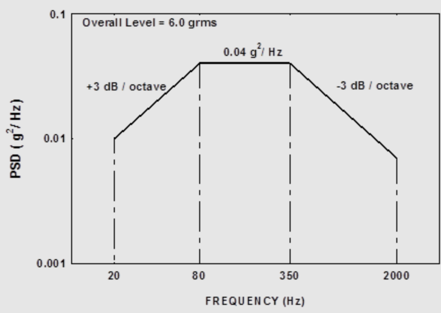

navmat = pd.read_csv('https://info.endaq.com/hubfs/navmat-p-9492.csv',delimiter='\t',header=None,index_col=0,names=['Random'])
navmat.index.name='Time (s)'

navmat['Add 2g @ 100 Hz'] = navmat.Random + 2*np.sin(2*np.pi*100 * navmat.index)
navmat['Add 2g @ 200 Hz'] = navmat.Random + 2*np.sin(2*np.pi*200 * navmat.index)
navmat['Add 2g @ 400 Hz'] = navmat.Random + 2*np.sin(2*np.pi*400 * navmat.index)
navmat

	Random	Add 2g @ 100 Hz	Add 2g @ 200 Hz	Add 2g @ 400 Hz
Time (s)
0.000000	-8.698490e-07	-8.698490e-07	-8.698490e-07	-8.698490e-07
0.000038	8.459350e-07	4.793334e-02	9.583830e-02	1.914556e-01
0.000076	1.871620e-06	9.583932e-02	1.914566e-01	3.811528e-01
0.000114	3.444110e-06	1.436908e-01	2.866355e-01	5.673498e-01
0.000153	6.051080e-06	1.914608e-01	3.811570e-01	7.483369e-01
...	...	...	...	...
9.999847	3.435810e-02	-1.571110e-01	-3.468213e-01	-7.140265e-01
9.999886	3.562460e-02	-1.080109e-01	-2.509046e-01	-5.315224e-01
9.999924	1.458970e-02	-8.125498e-02	-1.768794e-01	-3.665897e-01
9.999962	1.604150e-02	-3.183180e-02	-7.967766e-02	-1.751775e-01
10.000000	-2.424250e-04	-2.424250e-04	-2.424250e-04	-2.424250e-04

262144 rows × 4 columns

endaq.plot.rolling_min_max_envelope(navmat, plot_as_bars=True, desired_num_points=500, opacity=0.8)

endaq.plot.around_peak(navmat, num=1000)

FFTs

fft = welch_fft(navmat, bin_width=1)

fig = px.line(fft[20:2000])
fig.update_layout(
    title_text='NAVMAT P-9492 FFT (1 Hz Bin Width)',
    yaxis_title_text='Acceleration (g)',
    xaxis_title_text='Frequency (Hz)',
    xaxis_type='log',
    yaxis_type='log',
    legend_title_text=''
)

Now let’s demonstrate the trouble with FFTs by varying the length of time we’ll use and the bin width/resolution in the FFT.

bins = ['1/T', 1, 10]
times = [1.0, 10]

ffts = pd.DataFrame()
for bin in bins:
  for time in times:
    bin_t = bin
    if bin=='1/T':
      bin_t = 1/time
    fft = welch_fft(navmat[:time], bin_width=bin_t)
    fft = fft[20:2000].reset_index().melt(id_vars='frequency (Hz)')
    fft['Time'] = time
    fft['Bin Width'] = bin

    ffts = pd.concat([ffts,fft])

ffts

	frequency (Hz)	variable	value	Time	Bin Width
0	20.000229	Random	0.288549	1.0	1/T
1	21.000240	Random	0.169284	1.0	1/T
2	22.000252	Random	0.099324	1.0	1/T
3	23.000263	Random	0.101153	1.0	1/T
4	24.000275	Random	0.100844	1.0	1/T
...	...	...	...	...	...
787	1950.319916	Add 2g @ 400 Hz	0.388329	10.0	10
788	1960.321557	Add 2g @ 400 Hz	0.369708	10.0	10
789	1970.323197	Add 2g @ 400 Hz	0.335365	10.0	10
790	1980.324838	Add 2g @ 400 Hz	0.378497	10.0	10
791	1990.326478	Add 2g @ 400 Hz	0.346982	10.0	10

104548 rows × 5 columns

fig = px.line(
    ffts,
    x='frequency (Hz)',
    y='value',
    color='variable',
    log_y=True,
    log_x=True,
    facet_row='Time',
    facet_col='Bin Width',
    title='FFTs: Acceleration (g) vs Frequency (Hz)',
    labels={'value':'',
            'frequency (Hz)':'',
            'variable':''}

)
fig.update_layout(width=800,height=600)
fig.show(renderer='svg')

Our peaks stay consistent around the 2g we’d expect… but what is happening with the other frequency content!?

PSDs

psd = endaq.calc.psd.welch(navmat,bin_width=1)

fig = px.line(psd[20:2000])
fig.update_layout(
    title_text='NAVMAT P-9492 PSD (1 Hz Bin Width)',
    yaxis_title_text='Acceleration (g^2/Hz)',
    xaxis_title_text='Frequency (Hz)',
    xaxis_type='log',
    yaxis_type='log',
    legend_title_text=''
)

Now let’s do the same comparison of PSDs

psds = pd.DataFrame()
for bin in bins:
  for time in times:
    bin_t = bin
    if bin=='1/T':
      bin_t = 1/time
    psd = endaq.calc.psd.welch(
        navmat[:time], bin_width=bin_t)
    psd = psd[20:2000].reset_index().melt(id_vars='frequency (Hz)')
    psd['Time'] = time
    psd['Bin Width'] = bin

    psds = pd.concat([psds,psd])

fig = px.line(
    psds,
    x='frequency (Hz)',
    y='value',
    color='variable',
    log_y=True,
    log_x=True,
    facet_row='Time',
    facet_col='Bin Width',
    title='PSDs: Acceleration (g^2/Hz) vs Frequency (Hz)',
    labels={'value':'',
            'frequency (Hz)':'',
            'variable':''}

)
fig.update_layout(width=800,height=600)
fig.show(renderer='svg')

The peak at those sine tones decrease yet the bin width was wider and that sine tone was at one single frequency… so it is less dense. But then the other random/broadband levels are consistent regardless of our length of time or frequency resolution.

PSD Frequency Resolution and Octave Spacing

psd_coarse = endaq.calc.psd.welch(navmat,bin_width=10)

fig = px.line(psd_coarse[20:2000])
fig.update_layout(
    title_text='NAVMAT P-9492 PSD (10 Hz Bin Width)',
    yaxis_title_text='Acceleration (g^2/Hz)',
    xaxis_title_text='Frequency (Hz)',
    xaxis_type='log',
    yaxis_type='log',
    legend_title_text=''
)

Convert to an octave spaced PSD with to_octave() docs.

psd = endaq.calc.psd.welch(navmat,bin_width=1)
oct_psd = endaq.calc.psd.to_octave(psd,fstart=20,octave_bins=3)

fig = px.line(oct_psd[:2000])
fig.update_layout(
    title_text='NAVMAT P-9492 PSD 1/3 Octave',
    yaxis_title_text='Acceleration (g^2/Hz)',
    xaxis_title_text='Frequency (Hz)',
    xaxis_type='log',
    yaxis_type='log',
    legend_title_text='',
    template='endaq_light'
)

/usr/local/lib/python3.7/dist-packages/endaq/calc/psd.py:161: RuntimeWarning:

empty frequency bins in re-binned PSD; original PSD's frequency spacing is too coarse

Cumulative Sum from PSD

cum_rms = endaq.calc.psd.welch(navmat,bin_width=1, scaling='parseval').cumsum()**0.5

fig = px.line(cum_rms[10:2000])
fig.update_layout(
    title_text='NAVMAT P-9492 PSD with Added Sine Tone',
    yaxis_title_text='Cumulative Acceleration RMS (g)',
    xaxis_title_text='Frequency (Hz)',
    xaxis_type='log',
    legend_title_text=''
)

Random Vibration Examples

Bearing

The first example was the topic of our blog on top 12 vibration metrics.

bearing = pd.read_csv('https://info.endaq.com/hubfs/Plots/bearing_data.csv', index_col=0)

endaq.plot.rolling_min_max_envelope(bearing, plot_as_bars=True, desired_num_points=500, opacity=0.8)

psd = endaq.calc.psd.welch(bearing,bin_width=10)

fig = px.line(psd)
fig.update_layout(
    title_text='Bearing Vibration',
    yaxis_title_text='Acceleration (g^2/Hz)',
    xaxis_title_text='Frequency (Hz)',
    xaxis_type='log',
    yaxis_type='log',
    legend_title_text='',
    template='endaq_light'
)

Car Engine

During a morning commute (many years ago) I mounted an enDAQ sensor to the car’s engine.

engine = endaq.ide.to_pandas(endaq.ide.get_doc('https://info.endaq.com/hubfs/data/Commute.ide').channels[8])
engine = endaq.calc.filters.butterworth(engine,low_cutoff=1)

endaq.plot.rolling_min_max_envelope(engine, plot_as_bars=True, desired_num_points=500, opacity=0.8)

psd = endaq.calc.psd.welch(engine,bin_width=1)

fig = px.line(psd)
fig.update_layout(
    title_text='VIbration of an Engine',
    yaxis_title_text='Acceleration (g^2/Hz)',
    xaxis_title_text='Frequency (Hz)',
    xaxis_type='log',
    yaxis_type='log',
    legend_title_text='',
    template='endaq_light'
)

Here we’ll use the octave_spectrogram() (see docs) to generate a spectrogram with log spaced frequency bins.

data, fig = endaq.plot.octave_spectrogram(engine[['Z']], window=2, bins_per_octave=24, freq_start= 20, max_freq=100)
fig.show()

/usr/local/lib/python3.7/dist-packages/endaq/calc/psd.py:161: RuntimeWarning:

empty frequency bins in re-binned PSD; original PSD's frequency spacing is too coarse

data = 10 ** (data/10)

fig = px.line(data[data.index<500].idxmax())
fig.update_layout(
    title_text="Moving Peak Frequency",
    xaxis_title_text="",
    yaxis_title_text="Peak Frequency (Hz)",
    showlegend=False
)
fig.show()

Quick Poll - What FFT Support Should We Add?

Remember this is an open source library you can view, comment and “react” to feature requests and bug reports. Here is an “issue” created to document this need to add some FFT support.

Simple Shock Response Spectrums

We’ll look at two datasets in our blog on pseudo velocity.

Punching Bag

punch = endaq.ide.to_pandas(endaq.ide.get_doc('https://info.endaq.com/hubfs/data/Punching-Bag.ide').channels[8], time_mode='seconds')
punch = punch - punch.median()

endaq.plot.rolling_min_max_envelope(punch, plot_as_bars=True, desired_num_points=500, opacity=0.8)

fig = endaq.plot.around_peak(punch, num=1000, leading_ratio=0.2)
fig.update_layout(
    xaxis_title_text='',
    yaxis_title_text='Acceleration (g)',
    legend_title_text=''
)

First determine the frequency bins to calculate it at.

freqs = endaq.calc.utils.logfreqs(punch[29:30], bins_per_octave=12)

Now perform the shock response spectrum calculation for those frequencies.

srs_punch = endaq.calc.shock.shock_spectrum(punch[29:30], freqs=freqs, damp=0.05, mode='srs')

Now plot!

fig = px.line(srs_punch)
fig.update_layout(
    title_text='Shock Response Spectrum (SRS) of Punching Bag',
    xaxis_title_text="Natural Frequency (Hz)",
    yaxis_title_text="Peak Acceleration (g)",
    legend_title_text='',
    xaxis_type="log",
    yaxis_type="log",
  )

Repeat for the PVSS.

pvss_punch = endaq.calc.shock.shock_spectrum(punch[29:30], freqs=freqs, damp=0.05, mode='pvss')
pvss_punch = pvss_punch*9.81*39.37 #convert to in/s

fig = px.line(pvss_punch)
fig.update_layout(
    title_text='Psuedo Velocity Shock Spectrum (PVSS) of Punching Bag',
    xaxis_title_text="Natural Frequency (Hz)",
    yaxis_title_text="Psuedo Velocity (in/s)",
    legend_title_text='',
    xaxis_type="log",
    yaxis_type="log",
  )

MIL-S-901D Barge Shock

barge = pd.read_csv('https://info.endaq.com/hubfs/data/mil-s-901d-barge.csv', names=['Time (s)','Accel (g)']).set_index('Time (s)')
barge = barge - barge.median()

endaq.plot.rolling_min_max_envelope(barge, plot_as_bars=True, desired_num_points=500, opacity=0.8)

fig = endaq.plot.around_peak(barge, num=1000, leading_ratio=0.2)
fig.update_layout(
    xaxis_title_text='',
    yaxis_title_text='Acceleration (g)',
    showlegend=False
)

First determine the frequency bins to calculate it at. Here though we will specify an initial frequency of one lower than the duration.

freqs = endaq.calc.utils.logfreqs(barge, init_freq=1, bins_per_octave=12)

/usr/local/lib/python3.7/dist-packages/endaq/calc/utils.py:54: RuntimeWarning:

the data's duration is too short to accurately represent an initial frequency of 1.000 Hz

Now perform the shock response spectrum calculation for those frequencies.

srs_barge = endaq.calc.shock.shock_spectrum(barge, freqs=freqs, damp=0.05, mode='srs')

Now plot!

fig = px.line(srs_barge)
fig.update_layout(
    title_text='Shock Response Spectrum (SRS) of MIL-S-901 Barge',
    xaxis_title_text="Natural Frequency (Hz)",
    yaxis_title_text="Peak Acceleration (g)",
    legend_title_text='',
    xaxis_type="log",
    yaxis_type="log",
  )

Repeat for the PVSS.

pvss_barge = endaq.calc.shock.shock_spectrum(barge, freqs=freqs, damp=0.05, mode='pvss')
pvss_barge = pvss_barge*9.81*39.37 #convert to in/s

fig = px.line(pvss_barge)
fig.update_layout(
    title_text='Psuedo Velocity Shock Spectrum (PVSS) of MIL-S-901 Barge',
    xaxis_title_text="Natural Frequency (Hz)",
    yaxis_title_text="Psuedo Velocity (in/s)",
    legend_title_text='',
    xaxis_type="log",
    yaxis_type="log",
  )

Compare

srs_punch = srs_punch[['Z (100g)']].reset_index().melt(id_vars='frequency (Hz)')
srs_punch['variable'] = 'Punching Bag (80g Peak)'

srs_barge = srs_barge.reset_index().melt(id_vars='frequency (Hz)')
srs_barge['variable'] = 'MIL-S-901 (600g Peak)'

srs_combined = pd.concat([srs_punch, srs_barge])

fig = px.line(
    srs_combined,
    x='frequency (Hz)',
    y='value',
    color='variable'
)
fig.update_layout(
    title_text='Shock Response Spectrum (SRS) Comparison',
    xaxis_title_text="Natural Frequency (Hz)",
    yaxis_title_text="Peak Acceleration (g)",
    legend_title_text='',
    xaxis_type="log",
    yaxis_type="log",
  )

pvss_punch = pvss_punch[['Z (100g)']].reset_index().melt(id_vars='frequency (Hz)')
pvss_punch['variable'] = 'Punching Bag (80g Peak)'

pvss_barge = pvss_barge.reset_index().melt(id_vars='frequency (Hz)')
pvss_barge['variable'] = 'MIL-S-901 (600g Peak)'

pvss_combined = pd.concat([pvss_punch, pvss_barge])

fig = px.line(
    pvss_combined,
    x='frequency (Hz)',
    y='value',
    color='variable'
)
fig.update_layout(
    title_text='Psuedo Velocity Shock Spectrum (PVSS) Comparison',
    xaxis_title_text="Natural Frequency (Hz)",
    yaxis_title_text="Psuedo Velocity (in/s)",
    legend_title_text='',
    xaxis_type="log",
    yaxis_type="log",
  )

Peak Finding

bumps = endaq.ide.to_pandas(endaq.ide.get_doc('https://info.endaq.com/hubfs/data/Robotic-Bumps.ide').channels[80], time_mode='seconds')
bumps = bumps - bumps.median()

fig = endaq.plot.rolling_min_max_envelope(bumps, plot_as_bars=True, desired_num_points=500, opacity=0.8)
fig.show()

Now we’ll use SciPy’s find_peaks function to isolate the major events.

peak_times, _ = scipy.signal.find_peaks(
    x = bumps['Y (40g)'].abs(),
    distance = 5 / endaq.calc.utils.sample_spacing(bumps), #spaced 5 seconds apart
    height = 8
)

Let’s add them to the previous plot!

fig.add_trace(go.Scatter(
    x=bumps.iloc[peak_times].index,
    y=bumps.iloc[peak_times]['Y (40g)'],
    name='Peaks',
    mode='markers',
    marker_size=10,
    marker_color='#D72D2D'
))
fig.show()

Now let’s plot the peak event with the identified peak.

fig = endaq.plot.around_peak(bumps, num=1000, leading_ratio=0.2)
fig.update_layout(
    xaxis_title_text='',
    yaxis_title_text='Acceleration (g)',
    legend_title_text=''
)
fig.add_trace(go.Scatter(
    x=[bumps.iloc[peak_times[2]].name],
    y=[bumps.iloc[peak_times[2]]['Y (40g)']],
    name='Peak',
    mode='markers',
    marker_size=10,
    marker_color='#D72D2D'
))
fig.show()

PVSS of Full Time History

freqs = endaq.calc.utils.logfreqs(bumps, init_freq=1, bins_per_octave=12)
pvss_bumps = endaq.calc.shock.shock_spectrum(bumps, freqs=freqs, damp=0.05, mode='pvss')
pvss_bumps = pvss_bumps*9.81*39.37 #convert to in/s

fig = px.line(pvss_bumps)
fig.update_layout(
    title_text='Psuedo Velocity Shock Spectrum (PVSS) of Robotic "Bumps"',
    xaxis_title_text="Natural Frequency (Hz)",
    yaxis_title_text="Psuedo Velocity (in/s)",
    legend_title_text='',
    xaxis_type="log",
    yaxis_type="log",
  )

You may be surprised to see the X axis actually had higher peak velocities than the Y axis because of where the frequency content lies!

Loop Through All Peaks

pvss_all = pd.DataFrame()

for peak in peak_times:
  freqs = endaq.calc.utils.logfreqs(bumps.iloc[peak-1000:peak+4000], init_freq=1, bins_per_octave=12)
  pvss = endaq.calc.shock.shock_spectrum(bumps.iloc[peak-1000:peak+4000], freqs=freqs, damp=0.05, mode='pvss')*9.81*39.37 #convert to in/s
  pvss = pvss.reset_index().melt(id_vars='frequency (Hz)')
  pvss['Peak'] = np.abs(bumps.iloc[peak]['Y (40g)'])
  pvss['Time'] = bumps.index[peak]

  pvss_all = pd.concat([pvss_all,pvss])

pvss_all['Peak'] = np.round(pvss_all['Peak'],1)
fig = px.line(
    pvss_all,
    x='frequency (Hz)',
    y='value',
    facet_col='variable',
    color='Peak',
    hover_data=['value','Time'],
    log_x=True,
    log_y=True,
    title='Comparison of PVSS for Each Event',
    labels={'value':'Peak Pseudo Velocity (in/s)','frequency (Hz)':''}
)
fig.for_each_annotation(lambda a: a.update(text=a.text.split("=")[-1]))
fig.show()

Notice how the peak at 23.5g has a pseudo velocity about 1/2 that compared to the peak at virtually all the other events, including the one at 12.8g.

Preview of Batch

This is currently available, see docs, but we are working on a few bug fixes and improved functionality. This module allows you to batch process many IDE (only works for our sensors for now).

In a seperate document I first executed the following code to gather all the .IDE files I wanted to analyze (I hide the actual folder name). ~~~python import glob directory = r“C:\Users\shanly\enDAQ-Notebooks…”+“\”

files = glob.glob(directory+“.ide”) #get all the files in that directory with a .ide extension ~~~

Then with this list of files, I performed the batch operation with the following. ~[STRIKEOUT:python calc_output = ( endaq.batch.GetDataBuilder(accel_highpass_cutoff=1) .add_psd(freq_bin_width=1) .add_metrics() .aggregate_data(files) ) file_data = calc_output.dataframes]~

Then I saved the output dataframes of interest to pickles that I will load next! ~[STRIKEOUT:python file_data[‘psd’].to_pickle(‘batch_psd.pkl’, protocol=4) file_data[‘metrics’].to_pickle(‘batch_metrics.pkl’, protocol=4)]~

Note that I obscured the actual filenames (that would have contained the path) with these lines prior to saving. ~[STRIKEOUT:python file_data[‘metrics’].filename = file_data[‘metrics’].filename.str.split(‘\’).str[-1].str.split(‘.IDE’).str[0] file_data[‘psd’].filename = file_data[‘psd’].filename.str.split(‘\’).str[-1].str.split(‘.IDE’).str[0]]~

Metrics

metrics = pd.read_pickle('https://info.endaq.com/hubfs/data/batch_metrics.pkl')
metrics

	filename	calculation	axis	value	serial number	start time
0	DAQ11409_000061	RMS Acceleration	X (40g)	0.050146	11409	2021-10-27 17:33:19.722259
1	DAQ11409_000061	RMS Velocity	X (40g)	44.938216	11409	2021-10-27 17:33:19.722259
2	DAQ11409_000061	RMS Displacement	X (40g)	5.836992	11409	2021-10-27 17:33:19.722259
3	DAQ11409_000061	Peak Absolute Acceleration	X (40g)	0.906830	11409	2021-10-27 17:33:19.722259
4	DAQ11409_000061	Peak Pseudo Velocity Shock Spectrum	X (40g)	0.002361	11409	2021-10-27 17:33:19.722259
...	...	...	...	...	...	...
148258	DAQ11409_005795	RMS Angular Velocity	X	1.541428	11409	2021-11-16 19:52:53.617858
148259	DAQ11409_005795	RMS Angular Velocity	Y	0.344340	11409	2021-11-16 19:52:53.617858
148260	DAQ11409_005795	RMS Angular Velocity	Z	0.057123	11409	2021-11-16 19:52:53.617858
148261	DAQ11409_005795	Average Temperature	Pressure/Temperature:00	15.580078	11409	2021-11-16 19:52:53.617858
148262	DAQ11409_005795	Average Temperature	Control Pad Pressure	89.527103	11409	2021-11-16 19:52:53.617858

148263 rows × 6 columns

metrics.calculation.unique()

array(['RMS Acceleration', 'RMS Velocity', 'RMS Displacement',
       'Peak Absolute Acceleration',
       'Peak Pseudo Velocity Shock Spectrum', 'RMS Angular Velocity',
       'Average Temperature'], dtype=object)

fig = px.scatter(
    metrics[metrics.calculation.isin(['RMS Acceleration',
                                      'RMS Displacement',
                                      'Peak Absolute Acceleration'])],
    x='start time',
    y='value',
    facet_col='calculation',
    facet_col_wrap=1,
    color='axis',
    labels={'value':'',
            'start time':'',
            'axis':''
           },
    hover_data=['filename']
)
fig.update_layout(height=600)
fig.for_each_annotation(lambda a: a.update(text=a.text.split("=")[-1]))
fig.update_yaxes(matches=None)
fig.show()

PSDs

psd = pd.read_pickle('https://info.endaq.com/hubfs/data/batch_psd.pkl')
psd

	filename	axis	frequency (Hz)	value	serial number	start time
0	DAQ11409_000061	X (40g)	0.000000	7.402487e-10	11409	2021-10-27 17:33:19.722259
1	DAQ11409_000061	Y (40g)	0.000000	2.419061e-08	11409	2021-10-27 17:33:19.722259
2	DAQ11409_000061	Z (40g)	0.000000	4.245836e-09	11409	2021-10-27 17:33:19.722259
3	DAQ11409_000061	Resultant	0.000000	2.917670e-08	11409	2021-10-27 17:33:19.722259
4	DAQ11409_000061	X (40g)	1.003505	4.808626e-09	11409	2021-10-27 17:33:19.722259
...	...	...	...	...	...	...
2876195	DAQ11409_005795	Resultant	124.448957	7.143454e-08	11409	2021-11-16 19:52:53.617858
2876196	DAQ11409_005795	X (40g)	125.452578	1.768300e-08	11409	2021-11-16 19:52:53.617858
2876197	DAQ11409_005795	Y (40g)	125.452578	3.348997e-09	11409	2021-11-16 19:52:53.617858
2876198	DAQ11409_005795	Z (40g)	125.452578	5.949278e-08	11409	2021-11-16 19:52:53.617858
2876199	DAQ11409_005795	Resultant	125.452578	8.052478e-08	11409	2021-11-16 19:52:53.617858

2876200 rows × 6 columns

Now we want to aggregate this see how things changed over time. So we’ll round the frequency values and focus on one axis. For readability we’ll also make a new column that will display time into the test in days.

psd['frequency (Hz)'] = np.round(psd['frequency (Hz)'] ,0)
psd['start time'] = pd.to_datetime(psd['start time'])
psd['Test Day'] = psd['start time']-psd['start time'].iloc[0]
psd['Test Day'] = np.round(psd['Test Day'].dt.total_seconds()/60/60/24,3)

psd_y = psd[psd.axis=='Y (40g)'].copy()
psd_y

	filename	axis	frequency (Hz)	value	serial number	start time	Test Day
1	DAQ11409_000061	Y (40g)	0.0	2.419061e-08	11409	2021-10-27 17:33:19.722259	0.000
5	DAQ11409_000061	Y (40g)	1.0	2.557175e-07	11409	2021-10-27 17:33:19.722259	0.000
9	DAQ11409_000061	Y (40g)	2.0	2.522567e-06	11409	2021-10-27 17:33:19.722259	0.000
13	DAQ11409_000061	Y (40g)	3.0	1.247001e-06	11409	2021-10-27 17:33:19.722259	0.000
17	DAQ11409_000061	Y (40g)	4.0	7.596711e-08	11409	2021-10-27 17:33:19.722259	0.000
...	...	...	...	...	...	...	...
2876181	DAQ11409_005795	Y (40g)	121.0	1.037411e-08	11409	2021-11-16 19:52:53.617858	20.097
2876185	DAQ11409_005795	Y (40g)	122.0	6.082880e-09	11409	2021-11-16 19:52:53.617858	20.097
2876189	DAQ11409_005795	Y (40g)	123.0	5.461760e-09	11409	2021-11-16 19:52:53.617858	20.097
2876193	DAQ11409_005795	Y (40g)	124.0	4.885745e-09	11409	2021-11-16 19:52:53.617858	20.097
2876197	DAQ11409_005795	Y (40g)	125.0	3.348997e-09	11409	2021-11-16 19:52:53.617858	20.097

719050 rows × 7 columns

2D Waterfall

Let’s see how the PSD changes over time in a 2D plot with a bunch of lines (one per time). To help with the visualization we first need to get a bunch of colors to map to.

from plotly import colors
num_colors = len(psd_y[psd_y['Test Day']<1]['Test Day'].unique())
color_steps = colors.sample_colorscale(px.colors.sequential.Turbo, num_colors)

Now we can make the plot!

fig = px.line(
    psd_y[psd_y['Test Day']<1],
    x='frequency (Hz)',
    y='value',
    color='Test Day',
    hover_data=['filename','start time'],
    color_discrete_sequence = color_steps
)
fig.update_layout(
    xaxis_title_text='Frequency (Hz)',
    yaxis_title_text='Acceleration (g^2/Hz)',
    legend_title_text='',
    legend_y=-0.7,
    height=800,
    xaxis_type='log',
    yaxis_type='log',
    template='endaq_light'
)

3D Waterfall

I know everyone wants to see the 3D view…

fig = px.line_3d(
    psd_y[psd_y['Test Day']<1],
    x='frequency (Hz)',
    z='value',
    y='Test Day',
    color='Test Day',
    hover_data=['filename','start time'],
    color_discrete_sequence = color_steps,
    log_x=True,
    log_z=True,
    labels={'value':'Acceleration (g^2/Hz)','frequency (Hz)':'Frequency (Hz)'}
)
fig.update_layout(
    title_text='3D Waterfall Plot',
    showlegend = False,
    margin=dict(l=20, r=20, t=20, b=20),
    template='endaq_light'
)

fig.write_html('3d-waterfall.html',include_plotlyjs='cdn')

Animation

This let’s us create animations which I’ll first do on the first day’s worth of data.

fig = px.line(
    psd_y[psd_y['Test Day']<1],
    x='frequency (Hz)',
    y='value',
    animation_frame='Test Day',
    hover_data=['filename','start time']
)
fig.update_layout(
    xaxis_title_text='Frequency (Hz)',
    yaxis_title_text='Acceleration (g^2/Hz)',
    legend_title_text='',
    xaxis_type='log',
    yaxis_type='log',
)

That’s pretty cool! But we’ll notice that the animation moves outside the inital bounds pretty quickly. So let’s first find an easy way to calculate these metrics of max/min/median per frequency bin.

psd_pivot = psd_y.pivot(index='frequency (Hz)', columns='start time', values='value')
psd_pivot

start time	2021-10-27 17:33:19.722259	2021-10-27 17:38:21.101715	2021-10-27 17:43:22.482452	2021-10-27 17:48:23.870605	2021-10-27 17:53:25.254699	2021-10-27 17:58:26.638977	2021-10-27 18:03:28.009857	2021-10-27 18:08:29.389068	2021-10-27 18:13:30.775756	2021-10-27 18:18:32.146697	2021-10-27 18:23:33.514129	2021-10-27 18:28:34.893768	2021-10-27 18:33:36.268646	2021-10-27 18:38:37.657501	2021-10-27 18:43:39.036804	2021-10-27 18:48:40.431610	2021-10-27 18:53:41.812469	2021-10-27 18:58:43.190490	2021-10-27 19:03:44.574890	2021-10-27 19:08:45.954772	2021-10-27 19:13:47.342895	2021-10-27 19:18:48.719848	2021-10-27 19:23:50.096343	2021-10-27 19:28:51.476501	2021-10-27 19:33:52.856201	2021-10-27 19:38:54.239196	2021-10-27 19:43:55.622436	2021-10-27 19:48:57.017181	2021-10-27 19:53:58.401855	2021-10-27 19:58:59.786193	2021-10-27 20:04:01.182495	2021-10-27 20:09:02.573852	2021-10-27 20:14:03.964660	2021-10-27 20:19:05.560089	2021-10-27 20:24:06.949493	2021-10-27 20:29:08.341552	2021-10-27 20:34:09.737091	2021-10-27 20:39:11.129425	2021-10-27 20:44:12.713470	2021-10-27 20:49:14.100280	...	2021-11-16 16:35:08.246185	2021-11-16 16:40:12.454956	2021-11-16 16:45:16.662902	2021-11-16 16:50:20.865539	2021-11-16 16:55:25.078521	2021-11-16 17:00:29.311737	2021-11-16 17:05:33.518707	2021-11-16 17:10:37.732543	2021-11-16 17:15:41.967681	2021-11-16 17:20:46.173339	2021-11-16 17:25:50.585174	2021-11-16 17:30:54.814361	2021-11-16 17:35:59.042205	2021-11-16 17:41:03.259735	2021-11-16 17:46:07.486053	2021-11-16 17:51:11.697174	2021-11-16 17:56:15.934448	2021-11-16 18:01:20.156829	2021-11-16 18:06:24.380767	2021-11-16 18:11:28.603668	2021-11-16 18:16:32.835784	2021-11-16 18:21:37.054992	2021-11-16 18:26:41.778625	2021-11-16 18:31:45.985595	2021-11-16 18:36:50.203430	2021-11-16 18:41:54.423553	2021-11-16 18:46:58.631286	2021-11-16 18:52:02.839935	2021-11-16 18:57:07.076232	2021-11-16 19:02:11.296142	2021-11-16 19:07:15.528411	2021-11-16 19:12:19.742004	2021-11-16 19:17:23.986328	2021-11-16 19:22:28.219085	2021-11-16 19:27:32.438873	2021-11-16 19:32:36.662109	2021-11-16 19:37:40.912109	2021-11-16 19:42:45.152252	2021-11-16 19:47:49.379699	2021-11-16 19:52:53.617858
frequency (Hz)
0.0	2.419061e-08	6.961451e-09	2.694621e-08	0.000004	0.000008	0.000003	0.000003	0.000003	0.000001	0.000002	0.000004	0.000005	0.000008	0.000003	0.000002	0.000003	0.000002	0.000002	0.000005	0.000002	0.000001	0.000003	9.199357e-07	0.000003	1.518771e-06	0.000002	0.000002	2.163578e-06	0.000008	0.000002	0.000004	3.760117e-06	8.331635e-07	0.000002	2.212025e-06	1.235489e-06	2.958984e-06	1.301514e-06	1.982634e-06	0.000005	...	0.000003	3.022666e-06	4.218103e-06	0.000008	3.078788e-06	0.000002	2.032640e-06	7.642987e-06	2.100572e-06	3.379650e-06	2.492302e-06	9.384487e-06	2.791448e-06	2.543345e-06	0.000002	2.078568e-06	8.132484e-07	2.838021e-06	0.000004	4.413651e-06	0.000002	6.958460e-06	0.000005	2.259085e-06	2.582262e-06	8.285179e-06	0.000004	7.115846e-06	1.923488e-06	1.178528e-06	0.000005	1.850663e-07	5.758527e-08	4.356333e-08	1.326678e-08	3.523284e-08	3.401198e-08	9.321506e-08	2.072132e-07	5.329716e-08
1.0	2.557175e-07	8.999609e-08	1.926265e-07	0.000034	0.000055	0.000041	0.000037	0.000020	0.000022	0.000016	0.000045	0.000052	0.000049	0.000039	0.000026	0.000032	0.000011	0.000027	0.000051	0.000038	0.000007	0.000015	1.105532e-05	0.000036	1.671067e-05	0.000023	0.000026	1.953543e-05	0.000087	0.000031	0.000041	4.049195e-05	1.907499e-05	0.000032	2.385972e-05	1.026427e-05	2.749858e-05	1.615311e-05	2.693152e-05	0.000080	...	0.000057	2.867848e-05	5.494686e-05	0.000059	1.791955e-05	0.000025	3.726021e-05	7.125737e-05	2.376242e-05	3.463165e-05	2.879028e-05	4.655712e-05	7.107180e-05	4.406466e-05	0.000065	4.128956e-05	1.860609e-05	4.077474e-05	0.000033	8.258510e-05	0.000014	7.395578e-05	0.000057	2.943697e-05	3.235613e-05	1.141953e-04	0.000103	5.089320e-05	3.296615e-05	2.210161e-05	0.000058	1.788990e-06	6.666895e-07	4.819046e-07	6.939725e-07	3.583268e-07	8.923644e-07	1.693514e-06	5.189828e-06	3.352921e-07
2.0	2.522567e-06	6.889837e-07	2.332143e-06	0.000208	0.000298	0.000202	0.000104	0.000118	0.000102	0.000077	0.000193	0.000266	0.000251	0.000146	0.000130	0.000145	0.000073	0.000150	0.000230	0.000155	0.000044	0.000097	4.346807e-05	0.000199	6.920640e-05	0.000099	0.000104	9.560500e-05	0.000549	0.000116	0.000247	3.122200e-04	1.225986e-04	0.000119	1.170403e-04	4.953305e-05	1.380503e-04	1.002347e-04	1.661748e-04	0.000339	...	0.000234	1.086385e-04	3.531844e-04	0.000271	1.440112e-04	0.000148	2.247540e-04	3.794856e-04	1.091585e-04	1.625495e-04	2.139703e-04	2.784456e-04	3.102676e-04	2.197761e-04	0.000248	2.685322e-04	7.470985e-05	2.238129e-04	0.000208	5.037352e-04	0.000094	5.531540e-04	0.000472	1.668488e-04	1.696425e-04	5.673354e-04	0.000513	3.158666e-04	1.340000e-04	1.496420e-04	0.000383	1.414038e-05	4.116737e-06	3.061537e-06	3.137081e-06	2.238157e-06	3.732002e-06	8.260310e-06	2.382195e-05	3.364408e-06
3.0	1.247001e-06	3.708911e-07	1.238390e-06	0.000122	0.000155	0.000151	0.000053	0.000066	0.000059	0.000041	0.000116	0.000133	0.000148	0.000081	0.000059	0.000073	0.000037	0.000056	0.000124	0.000073	0.000026	0.000069	3.026884e-05	0.000104	4.267918e-05	0.000057	0.000043	6.355741e-05	0.000216	0.000054	0.000132	1.861895e-04	6.389375e-05	0.000079	7.598246e-05	4.548199e-05	6.775841e-05	6.932025e-05	8.357926e-05	0.000180	...	0.000137	6.661549e-05	2.033306e-04	0.000178	1.262726e-04	0.000082	1.100094e-04	1.730692e-04	5.929123e-05	1.030920e-04	1.313220e-04	2.379084e-04	1.730239e-04	1.114687e-04	0.000104	1.285181e-04	3.582072e-05	1.165774e-04	0.000116	1.988762e-04	0.000067	2.372616e-04	0.000252	1.024006e-04	1.111846e-04	2.714036e-04	0.000222	2.389278e-04	9.763413e-05	8.946194e-05	0.000149	8.732022e-06	2.575371e-06	1.443267e-06	1.056115e-06	1.322230e-06	2.146535e-06	4.270818e-06	1.430278e-05	2.720061e-06
4.0	7.596711e-08	3.332906e-08	2.693014e-07	0.000026	0.000026	0.000032	0.000023	0.000020	0.000027	0.000012	0.000033	0.000023	0.000034	0.000020	0.000014	0.000018	0.000009	0.000019	0.000036	0.000024	0.000008	0.000022	9.036514e-06	0.000025	1.038904e-05	0.000017	0.000013	1.145624e-05	0.000039	0.000013	0.000038	3.526670e-05	1.801536e-05	0.000019	1.389114e-05	6.302247e-06	2.129335e-05	1.779139e-05	1.426981e-05	0.000043	...	0.000059	1.420008e-05	2.916908e-05	0.000033	1.532318e-05	0.000016	1.920946e-05	5.402916e-05	1.619829e-05	4.107995e-05	2.308721e-05	6.647677e-05	5.163262e-05	2.292783e-05	0.000037	3.134771e-05	8.408034e-06	2.837890e-05	0.000028	4.000348e-05	0.000018	5.138282e-05	0.000051	2.366792e-05	2.534139e-05	7.182962e-05	0.000081	5.186834e-05	2.924370e-05	2.360597e-05	0.000056	1.866866e-06	1.077818e-06	6.921128e-07	2.991976e-07	1.100801e-07	4.083279e-07	3.597081e-07	1.828241e-06	4.625317e-07
...	...	...	...	...	...	...	...	...	...	...	...	...	...	...	...	...	...	...	...	...	...	...	...	...	...	...	...	...	...	...	...	...	...	...	...	...	...	...	...	...	...	...	...	...	...	...	...	...	...	...	...	...	...	...	...	...	...	...	...	...	...	...	...	...	...	...	...	...	...	...	...	...	...	...	...	...	...	...	...	...	...
122.0	4.794718e-08	1.403580e-09	1.555955e-09	0.000002	0.000013	0.000017	0.000002	0.000003	0.000003	0.000002	0.000002	0.000006	0.000004	0.000002	0.000004	0.000009	0.000021	0.000020	0.000019	0.000007	0.000008	0.000006	6.404928e-06	0.000012	1.515504e-05	0.000012	0.000003	1.431891e-05	0.000008	0.000004	0.000003	2.263224e-06	1.028560e-05	0.000002	4.241913e-06	4.873168e-06	1.225941e-06	3.019433e-06	1.951890e-06	0.000002	...	0.000012	2.195231e-05	2.106803e-05	0.000012	1.830445e-05	0.000010	1.882487e-05	2.267166e-05	5.221777e-06	2.167978e-05	1.289279e-05	1.664051e-05	1.671418e-05	5.891856e-06	0.000015	1.482488e-05	1.265719e-05	1.252918e-05	0.000015	2.233010e-05	0.000008	1.701158e-05	0.000007	4.759324e-06	1.749558e-05	6.335562e-06	0.000006	2.069402e-05	1.063007e-05	7.831063e-06	0.000011	6.039101e-09	4.662815e-09	3.121494e-09	5.535294e-09	9.558629e-09	5.412999e-09	1.458804e-08	1.983171e-08	6.082880e-09
123.0	1.851752e-08	1.599072e-09	2.228003e-09	0.000002	0.000003	0.000003	0.000002	0.000002	0.000001	0.000001	0.000002	0.000002	0.000002	0.000001	0.000001	0.000003	0.000002	0.000003	0.000003	0.000001	0.000001	0.000003	2.084756e-06	0.000004	4.710479e-06	0.000002	0.000003	6.170386e-06	0.000003	0.000002	0.000003	2.033750e-06	2.567449e-06	0.000002	1.504151e-06	1.682195e-06	1.000708e-06	1.408385e-06	1.328178e-06	0.000002	...	0.000003	4.974716e-06	4.804490e-06	0.000006	4.564517e-06	0.000003	4.870139e-06	8.099777e-06	2.389564e-06	4.807188e-06	2.969390e-06	4.548254e-06	5.288451e-06	2.222343e-06	0.000004	3.728426e-06	3.989563e-06	4.845033e-06	0.000005	6.873294e-06	0.000002	5.049589e-06	0.000005	2.686271e-06	5.196398e-06	4.537091e-06	0.000005	6.886131e-06	3.704323e-06	2.606997e-06	0.000003	5.848638e-09	2.652969e-09	3.802013e-09	3.680023e-09	7.588366e-09	3.352630e-09	1.334295e-08	1.356523e-08	5.461760e-09
124.0	1.526794e-08	1.904395e-09	3.012694e-09	0.000003	0.000002	0.000004	0.000004	0.000002	0.000001	0.000002	0.000005	0.000003	0.000002	0.000001	0.000001	0.000002	0.000001	0.000003	0.000005	0.000008	0.000001	0.000003	5.319471e-07	0.000002	7.423440e-07	0.000001	0.000002	1.331505e-06	0.000003	0.000001	0.000002	1.107081e-06	1.698859e-06	0.000001	7.515144e-07	5.368396e-07	7.445584e-07	8.629774e-07	1.665465e-06	0.000002	...	0.000003	1.273982e-06	1.744378e-06	0.000003	2.006455e-06	0.000001	1.867671e-06	3.270818e-06	1.444862e-06	1.950836e-06	1.375152e-06	3.053077e-06	3.156415e-06	1.976571e-06	0.000003	1.392365e-06	9.572028e-07	1.487826e-06	0.000003	2.841553e-06	0.000002	2.921201e-06	0.000005	1.717473e-06	3.548734e-06	3.188935e-06	0.000002	3.984916e-06	1.677965e-06	2.226348e-06	0.000003	6.599701e-09	3.184131e-09	4.878153e-09	4.554283e-09	4.333788e-09	4.143943e-09	6.197127e-09	1.149195e-08	4.885745e-09
125.0	1.554448e-08	2.240702e-09	2.165436e-09	0.000003	0.000003	0.000004	0.000003	0.000002	0.000002	0.000003	NaN	0.000009	0.000005	0.000005	0.000002	0.000006	0.000002	0.000008	0.000019	0.000008	0.000003	0.000004	1.340032e-06	0.000005	1.828251e-06	0.000002	0.000002	1.030046e-06	0.000003	0.000003	0.000001	1.376330e-06	1.444470e-06	NaN	1.055394e-06	3.712440e-07	NaN	1.261323e-06	9.890634e-07	0.000003	...	0.000002	1.289565e-06	1.452126e-06	0.000002	1.357979e-06	0.000001	1.266668e-06	2.451592e-06	3.529851e-07	1.686731e-06	7.846670e-07	2.801990e-06	2.365513e-06	8.005016e-07	0.000002	1.181413e-06	1.090871e-06	2.218299e-06	0.000003	2.916531e-06	0.000001	2.456790e-06	0.000001	2.894886e-07	1.862269e-06	9.910348e-07	NaN	2.436740e-06	9.076316e-07	7.792794e-07	0.000002	4.828801e-09	3.057908e-09	2.959562e-09	2.461398e-09	5.281825e-09	4.169273e-09	6.557761e-09	5.647898e-09	3.348997e-09
126.0	NaN	NaN	NaN	NaN	NaN	NaN	NaN	NaN	NaN	NaN	NaN	NaN	NaN	NaN	NaN	NaN	NaN	NaN	NaN	NaN	NaN	0.000004	1.284312e-06	0.000004	1.629573e-06	0.000002	0.000001	8.839285e-07	0.000002	0.000003	NaN	8.535060e-07	6.206068e-07	NaN	8.059833e-07	1.717251e-07	NaN	6.507064e-07	5.962763e-07	0.000002	...	NaN	3.593515e-07	4.812013e-07	0.000001	3.284124e-07	NaN	2.777564e-07	6.396569e-07	NaN	6.206701e-07	NaN	6.462563e-07	6.047255e-07	NaN	NaN	3.570359e-07	3.670580e-07	6.375746e-07	0.000002	9.608136e-07	NaN	5.880341e-07	NaN	NaN	4.747024e-07	NaN	NaN	8.688151e-07	NaN	NaN	NaN	NaN	NaN	NaN	NaN	NaN	NaN	NaN	NaN	NaN

127 rows × 5703 columns

In this format computing the metric per frequency bin is pretty easy:

psd_pivot.max(axis=1)

frequency (Hz)
0.0      0.000018
1.0      0.000155
2.0      0.000933
3.0      0.000521
4.0      0.000139
           ...
122.0    0.000059
123.0    0.000016
124.0    0.000011
125.0    0.000019
126.0    0.000005
Length: 127, dtype: float64

Now we can loop through and add these lines to our animation and update it.

def add_line(df_stat,name,dash,color):
  fig.add_trace(go.Scatter(
    x=df_stat.index,
    y=df_stat.values,
    name=name,
    line_width=3,
    line_dash=dash,
    line_color=color
))

#Add max, min, median
for stat,dash,quant in zip(['Max','Min','Median'],
                           [None,None,'dash'],
                           [1.0,0.0,0.5]):
  df_stat = psd_pivot.quantile(quant, axis=1)
  add_line(df_stat,stat,dash,'#6914F0')

fig.update_layout(
    legend_y=-0.7
)
fig.show()

That’s a Wrap!

Hopefully you have enough to get started but if not remember we do offer services! And we will be working on more and more documentation and examples!

previous

Introduction to the enDAQ library

next

Quick Start Guide